Vector Calculus with Python
In this little example we want to calculate the magnetic vector potential and field for a given distribution of magnetic moments in 3D.
For the case of rather large grids we use the multiprocessing capabilities of the Python interpreter in the calculations.
Physics of Magnetism
We start out with a cylindrical distribution of magnetic moments. In the x>0 half plane these moments are pointing towards the positive z axis. In the other half plane in the opposite direction (see Eq. 1).
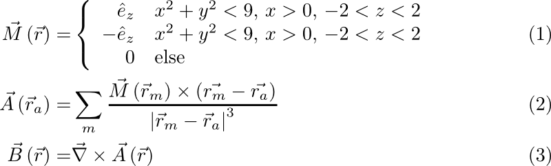
The magnetic vector potential A at the point ra is the sum or the integral of all present magnetic moments at positions rm (see Eq. 2). Finally the magnetic field B is given by the cross product of the Laplace operator with the vector potential.
The Script
The example script basically contains of two parts: The first part does the number crunching and the second part handles the data display:
#!/usr/bin/env python

import time
import sys
import os.path
import numpy
import mayavi.mlab
import Queue
import scipy.fftpack as fftpack
import multiprocessing

use_saved = False

def worker(myslice,q,A):
    if myslice[1] >= A.shape[1]:
        myslice[1] = A.shape[1]-1

    for a in range(myslice[0],myslice[1]):
        for b in range(A.shape[2]):
            for c in range(A.shape[3]):
                # ra is the position where the fields shall be
                # calculated.
                ra = numpy.array([x[a,b,c],y[a,b,c],z[a,b,c]])

                # Calculation of the vector potential and magnetic
                # field.
                a_sum = numpy.array((0,0,0),dtype='float')
                for d in range(m.shape[1]):
                    for e in range(m.shape[2]):
                        for f in range(m.shape[3]):
                            rm = numpy.array((x[d,e,f],y[d,e,f],z[d,e,f]))
                            M = m[:,d,e,f]
                            R = ra - rm
                            cube = betrag(R)**3
                            if cube.all() != 0:
                                a_sum += kreuzprodukt(M,R)/cube
                            else:
                                a_sum += numpy.zeros(3)
                A[:,a,b,c] = a_sum
                a_sum = numpy.zeros_like(a_sum)
    q.put((myslice,A))
    print "Finished!"
    return None

def partial(A,x=0):
    "Calculate partial derivative of a 3D pylab array along one axis."

    A_prime = numpy.zeros_like(A)
    l = list(A.shape)
    if len(l) > x: del l[x]

    for i in range(l[0]):
        for j in range(l[1]):
            if x==0:
                s = A[:,i,j].copy()
                A_prime[:,i,j] = fftpack.diff(s)
            elif x==1:
                s = A[i,:,j].copy()
                A_prime[i,:,j] = fftpack.diff(s)
            elif x==2:
                s = A[i,j,:].copy()
                A_prime[i,j,:] = fftpack.diff(s)
            else:
                raise ValueError, "No valid direction: %s" % x

    return A_prime

def betrag(a):
    return numpy.sqrt(abs(numpy.dot(a,a)))

def kreuzprodukt(a,b):
    tmp = numpy.array([
        a[1]*b[2] - a[2]*b[1],
        a[2]*b[0] - a[0]*b[2],
        a[0]*b[1] - a[1]*b[1]
    ])

    return tmp

data_file = "vector_field_A__switch_multiproc.npy"

# Queue for splitting the A compontents for passing to Threads
# Shape of queue elements: [begin,end]
try:
    max_threads = multiprocessing.cpu_count()
except Exception, e:
    print e
    max_threads = 2
print "No of Processes:", max_threads
# The coordinate grid
x,y,z = numpy.mgrid[-6:6:17j,-6:6:17j,-6:6:9j]

# The distribution of magnetic moments
m = numpy.array([
    numpy.zeros_like(x),
    numpy.zeros_like(y),
    numpy.select([x**2+y**2<9],[numpy.select([abs(z)<2,abs(z)>=2],[numpy.sign(x),0])])
])

if use_saved and os.path.isfile(data_file):
    A = numpy.load(data_file)
else:
    # The magnetic vector potential
    A = numpy.zeros_like(m)
    a = A.shape[1]/max_threads+1
    q = multiprocessing.Queue()
    for i in range(max_threads):
        myslice = [i*a,i*a+a]
        print myslice
        w = multiprocessing.Process(target=worker,args=(myslice,q,A))
        w.start()

    time.sleep(60)
    qItems = 0
    while multiprocessing.active_children():
        time.sleep(5)
        print q.qsize()
        try:
            myslice,A2 = q.get(True,timeout=10)
        except Exception,e:
            print "Caught exception:", e
            if qItems >=max_threads: break
        qItems += 1
        if myslice[1]> A.shape[1]: myslice[1] = A.shape[1]-1
        print myslice
        A[:,myslice[0]:myslice[1],:,:] = A2[:,myslice[0]:myslice[1],:,:].copy()
    numpy.save(data_file, A)

B = [
    partial(A[1],2) - partial(A[2],1),
    partial(A[2],0) - partial(A[0],2),
    partial(A[0],1) - partial(A[1],0)
]

mayavi.mlab.figure(size=(1280,800))
# Using plot functions
mayavi.mlab.quiver3d(x,y,z,m[0],m[1],m[2],name="Magnetic Moments")
mayavi.mlab.quiver3d(x,y,z,A[0],A[1],A[2],name="Vector Potential")
#mayavi.mlab.quiver3d(X,Y,Z,B[0],B[1],B[2],name="Magnetic Field")
# Creating the plot using the pipeline
src = mayavi.mlab.pipeline.vector_field(x,y,z,B[0],B[1],B[2],name="Magnetic Field")
mayavi.mlab.pipeline.vectors(src, mask_points=1, scale_factor=2.)
mayavi.mlab.pipeline.vector_cut_plane(src, mask_points=1, scale_factor=2.)

mayavi.mlab.outline()
mayavi.mlab.colorbar()
mayavi.mlab.show()
#mayavi.mlab.savefig("bla.png")
Parallel calculations
In order to speed up the computation time we use the multiprocessing module of Python to allow multiple interpreters to start and perform calculations.
After determining the number of available CPU cores (lines 95-98) the three dimensional array -- representing the region of interest -- is split into smaller slices (line 106).
An number of Processes equal to the number of cores are started (lines 107-108), if no file containing data is present, and calculate Eq. 2 on subslices (lines 27-40) passed as arguments to the Process contructor (line 107).
When all processes are finished (lines 110-111) the vector potential is saved (line 113).
Show the results
The magnetic field (Eq. 3) is calculated (lines 115-119) and displayed using Mayavi. The plot shows the magnetic moments (line 123), the vector potential (line 124) and the magnetic field (127-129), where Mayavi's pipelines are used to create a full vector field plot and a vector cut plane.
